Introduction
Most people have not read the Wells Report. But most people have an opinion on DeflateGate.
Even fewer have read the scientific portion of the Wells Report prepared by Exponent. Even fewer than that have read it critically. But again most people have an opinion on it.
So this is based on a critical reading of the Exponent report.
What specific evidence led the Exponent Investigators to their conclusion that someone had deflated the balls? Why do the Patriots still insist it must have been natural causes and the weather?
The Scene of the Crime
The primary evidence in this case was destroyed at halftime by the officials. This was not intentional. Simple physics tells us that if the amount of air (i.e. the number of air molecules) in the footballs does not change, and the temperature and dryness return to the state of the original measurements, the pressures will also return to the original pressure. Simply by taking 3 or 4 balls with the lowest pressure and locking them away in a cabinet for later analysis would have been sufficient to prove if there was any cheating going on. Instead, the officials pumped them up with more air, and sent them back out to the field.
For those of you who like Crime Scene Investigations, this would be like bystanders at an alleged crime scene taking a series of photos of what they think is evidence, then bundling up the critical evidence in a trash bag, and throwing it away to be incinerated.
What we have left is a set of pressure measurements taken while the balls were transitioning in temperature from the ball field to the warm locker room. There are questions of which gauges were used, how accurate the gauges were, the exact timing of the measurements, the climate in the locker room, and whether a comparison of the pressures in the Patriots balls to the Colts balls is even meaningful.
And then this was given to the Exponent Investigators to sift through to determine if a crime had even been committed.
The Investigative Report
The Exponent Investigators came up with a condemnation of the Patriots. Or at least the statement that it is “probable” that there was human intervention in the ball pressures, unless some other effect was discovered which might change their conclusion. And we are left with some serious questions as to how accurately their simulation of the Game-Day Scenario matched the actual conditions of the day.
The Exponent conclusion was based on an average pressure difference of just .2psi. In this situation, this amounts to a temperature difference of just 4oF. With a temperature change of 72F to 48F going from the locker room to the playing field respectively (and a corresponding pressure decrease by natural causes of 1.2psi) this seems small. The allowed starting range by the NFL rules is 12.5psi to 13.5psi. A .2psi difference is small compared to this range of pressure and is very unlikely to benefit a quarterback. It is even smaller than the .3psi inaccuracy of one of the gauges used in the measurements. But by doing a careful statistical analysis of the pressure, and using a simulated environment of the ball field and then the locker room the Investigators came up with this conclusion. The NFL leadership then decided “probable” was enough, and doled out a punishment to the Patriots, and singled out Tom Brady to suffer the brunt of that punishment.
The Denial of Guilt
The other side claims that there were other scientific factors missed by the Exponent Investigators, and there was just too much uncertainty in all these factors to come to any conclusion at all, and in fact the Patriots balls were close to the expected values. In addition their own investigation has failed to come up with a guilty party.
Our Review
We will look at some of those scientific factors which appear to have been missed by the Exponent Investigators, and how they might affect the conclusion.
We do this by looking at temperature primarily, but keeping track of the pressure. Temperature is a little more intuitive to people. According to the Ideal Gas Law, Pressure and Temperature are directly proportional to each other as long as the Volume and amount of air in the football does not change. In this particular case, a change in Temperature of 2oF results in a change in Pressure of about .1psi.
We will avoid discussion of most of the statistical calculations. These are very important to do, but do not really make sense unless you have all the significant factors identified and accounted for. They are also complex, and I generally find that if you are arguing because different interpretations of the statistics allow for different conclusions, the results are inconclusive anyway. There have been several different arguments about statistics in this case, and they do go either way, primarily because the result was so close statistically that Exponent could only issue a “probable” rating that there was a crime.
So we start with the Temperature Differential that was used to condemn the Patriots. This is shown in black. Then we look at problems with the report. Where they benefit the Patriots, they are shown in red, with an estimate of their size.
4oF (.2psi). The Critical Difference.
That is the average temperature difference between exonerating the Patriots, and condemning them. Just four degrees. The Exponent Investigators graph is shown below:
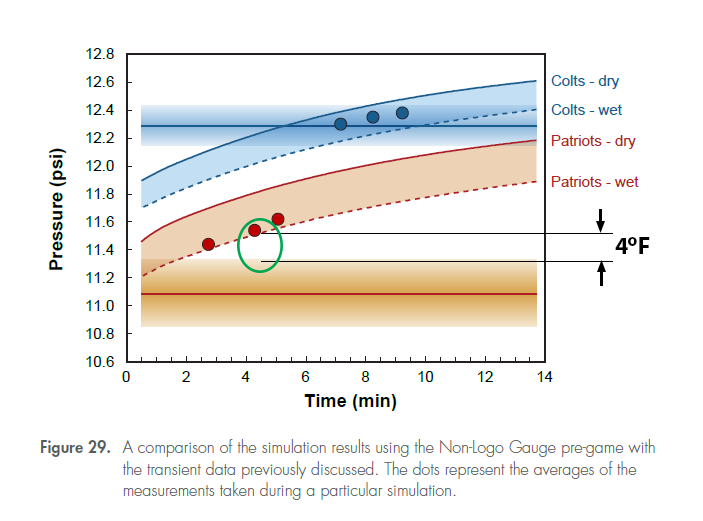
Figure 29 of the Wells report was meant to be the coup de grace for the Patriots that led the Exponent investigators to their conclusion that it was “probable” that human intervention caused the deflation of the footballs. The bottom line is the average of the Patriots football pressures, and the shaded area is the uncertainty (2-sigma) in the pressure as determined by the investigators. The wet-ball transient curve for the Patriots at 4.5 minutes lies about .2psi or 4oF above that uncertainty area. In fact, by this investigation, the transient curve pressure lies about four standard deviations above the mean. Assuming no uncertainty in the transient pressure curve as measured in the model, this is statistically significant, but still reasonably close, which is why the determination was “probable, and not a certainty.
The actual conclusion within the report after showing this graph is: “Therefore, subject to the discovery of an as yet unidentified and unexamined factor, the measurements recorded for the Patriots footballs on Game Day do not appear to be completely explainable based on natural causes alone.“
-1.5oF to -7.0oF. Gauge problems.
Referee Walt Anderson had two gauges in his bag when he measured the pressures in the balls before the game. He recalled using the “Logo” gauge, but wasn’t 100% certain. Both the Patriots and the Colts measured their own balls using their own gauges to be 12.5psi, and 13.0psi respectively. After that measurement, the balls from each team were brought to the floor of the officials locker room and left there. Walt Anderson a short time later measured the balls, and agreed with their measurements. The “Logo” gauge was later found to read about .3psi high, and the “non-Logo” gauge was about .07psi low. The temperature was estimated in the vicinity of where the balls were to be between 67F and 71F (probably a later measurement). There are a lot of permutations to choices of temperatures, gauges, balls, including switching gauges in the middle of the measurement.
Despite Walt Anderson’s recollections, the Exponent investigators concluded that it was likely that the non-Logo gauge was used. The Figure 29 graph in the previous section was done using the 71F temperature, and the “non-Logo” gauge.
A different conclusion could be reached by assuming that when the Patriots and Colts measured their own balls, they did so in locker rooms where the temperature was between 72F and 73F – the setting of the thermostat. (note — we do not know the settings of the thermostats in the Colts/Patriots locker rooms, however this was the setting in the officials locker room, and it stands to reason that it would be the same in the other locker rooms.) The referee’s measurement then confirms that they measured them at about the same temperature because the pressures were consistent by his gauge. ( the temperature of the balls in the officials locker room was then 66F-67F or 73F-74F for the logo or non-logo gauges respectively) Then let’s not worry about which gauge the referee used. The Colts gauge was later concluded by Exponent to be accurate, and that should be good enough. So instead of using a starting temperature of 71F, we should use a starting temperature of 72.5F.
This effectively brings the Patriot average pressure up by .075psi, or about 1.5F, closing the gap to 2.5F.
Another possibility is that Walt Anderson may have switched gauges in between measuring the two sets of footballs using the Logo gauge for the Patriots balls, and the non-Logo gauge for the Colts balls. This is a reasonable claim, especially since the Patriots have a protocol called “gloving” (rubbing the balls hard) which would have warmed the balls up prior to the Patriots final measurement of the balls. This could have set the Patriots balls at a pressure roughly .37psi lower than the Colts right from the opening gate, causing a 7oF shift in effective temperature of the Patriots balls.
The Exponent Investigators did do another graph depicting a starting temperature of 67F, and using the Logo gauge (Figure 27.). Some people claim there is a significant error in that graph setting which is described in a report in another blog by Steve McIntyre. Fixing that mistake may result in a similar effect as to the gauge switch described in the previous paragraph.
Unfortunately, there is a counter argument to every choice of which gauge was used for what, and we will never know the truth here. Rather than show a preference for one configuration or the other, the Wells Investigators need to rule out each possibility.
-1.0oF – 4.0oF. Evaporative cooling, and questionable climate control.
This will be confusing, and not very intuitive. It also requires a bit of advanced atmospheric physics and thermodynamics to understand.
An example of evaporative cooling is what happens when you sweat. A little bit of moisture on your skin cools it down. I think we all recognize that this cooling is dependent on humidity and wind speed. If it is humid, sweating is just not as effective cooling you down. Your body compensates and makes you sweat more. And a little bit of wind — a hand fan or a small breeze can be very refreshing and cooling.
The atmospheric terms we use here are wet-bulb temperature, and dry-bulb temperature. The dry-bulb temperature is the one we are used to, and we just call that the temperature. The web-bulb temperature is the temperature that something can cool down to if it gets wet. In fact to measure it, people will take a regular thermometer, wrap it in wet gauze, and wave it around in the air. If it is humid, the wet-bulb temperature will not be much cooler than the dry-bulb temperature, in fact at 100% humidity, it will be the same. In a low humidity situation, the temperature can be quite a bit lower, even as much as 20 or 30 degrees. Some of you may be familiar with a “swamp cooler”, or “evaporative cooler”, which in low humidity areas of the country can be a very effective cooling mechanism for a home using this principle.
Footballs can be cooled by evaporative cooling. Although Exponent never named it as such, we can see this cooling in their graphs. Here is their Fig 21:

Following the curves here, when the balls are brought to the field, they experience a temperature drop from 72F to 48F. The balls are dampened in this simulation by spraying them and wiping the water off with a cloth. Wet balls are subject to evaporative cooling. The humidity on the field was estimated to be 75%, so we can look up on a chart (a Psychrometric chart – see Appendix D) the wet-bulb temperature which would be 45F. This 3F drop in temperature corresponds to a .15psi drop in pressure, and this agrees with the difference in pressure between the dry balls and the wet balls as they descend in pressure seen in this figure.
When returning to the locker room, the balls come into a room where the Exponent Investigators claim the temperature matched that of the thermostat at 72F-73F, and the humidity was 20%. This is a very low humidity situation, but not uncommon in the winter. According to a Psychrometric chart, this corresponds to a wet-bulb temperature of 50F (see Appendix D). The final temperature for the “wet-ball” could then be somewhere between 72F (dry – 12.5psi), and 50F (wet with good air circulation – 11.4psi)! We overlaid the theoretical transient curves corresponding to these two extremes onto Figure 29, and that is shown here. (See Appendix C for details) The Exponent investigators don’t say anything about air circulation or climate control in general except that they tried to match the temperature and humidity of the air at the ball field, and at the locker room.
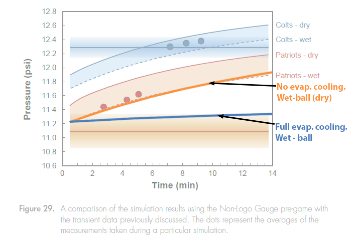
These theoretical transient curves are surprising, and perhaps even shocking! Walking into a room where the temperature rises from 48F to 72F, could cause very little increase in temperature or pressure in a wet football, as evaporative cooling takes over in the low humidity environment, and keeps the ball cool. Of course this requires good circulation — a wind.
Let me repeat that: The wet ball curve could be almost flat! Clearly this was not what Exponent measured! Their curve follows almost exactly a “dried” wet-ball curve, and ascends rapidly. Their measurement is not out of line with the theory, but the expectation would be that their curve would lie below the “dried” wet-ball curve, because the balls were wet, and evaporative cooling was observed to have an effect on footballs.
A theoretical derivation of these curves, and a thorough discussion of the Exponent measurement is found in Appendix C. It is clear from some of the Exponent charts that they had trouble with their climate control, in particular, controlling humidity and temperature in a consistent way. There is no discussion of this, nor an uncertainty in the their results due to these experimental factors which may have artificially increased the rate of rise of the ball pressure.
Also, in the Exponent report there was no discussion of air circulation in any of their simulations, but it may have played an significant role in the actual situation. Air circulation is both what helps warm the footballs, but also increases the rate of cooling from evaporation.
Is it possible the Exponent simulation day footballs were almost dry in the locker room? This goes against what was said by the officials who stated that some of the balls were “damp, but not waterlogged”. Do we have an estimate for the wind velocity and air circulation in the officials locker room? And did the Exponent Investigators provide circulation of that magnitude? Note, based on HVAC regulations for public locker rooms, it must have been at least .1mph (1.5 inches per second), and could have been 1-2mph if near a ventilation port.
So what do we do with this? Realistically, because the variation can be large here, the argument is incomplete until a more reliable measurement can be made, or the Exponent Investigators provide more explanation. One good step would have been for Exponent to calibrate their simulation chamber against the actual Officials locker room in Foxboro.
So right now, we keep it as a range. I do not expect it will be at the bottom of the range, nor at the top. I do expect that at least some drop in the experimental curve would occur if the climate control in the room was better (see Appendix C). That is the reason for at least 1oF lowering the curve.
-1oF to -5oF. Ball Bag Contact with the Cold Turf.
The bottom of the ball bag was sitting on AstroTurf which was sitting on a cold earth. Preceding game day, there were 18 days of January during which the Temperature rarely got out of the 20’s. On the day of the game, the temperature rose about 30 degrees, starting at 20F in the early morning to 50F at game time. We assume the ball bag is a quality athletic bag. Cooling is all about exposed surface areas, and the entire bottom of the bag was in contact with the turf for a couple hours leading up to halftime. Somewhere down below that bag, inside the turf is a boundary layer which was probably at 32F. The cooling power is brought to the surface through the wet nylon grass bristles as shown in the picture.

Now, this is pure conjecture, but it is hard to believe that there would not have been some effect here. 1 degree feels very conservative.
Imagine instead of a 50F day in January, this was a 90F day in May, where average temperatures in New England are in the 60’s. To cool off, you lay down on the ground in the shade where you can easily take advantage of the cool feel of the ground. The Physics is the same in January, however, the temperatures have been shifted by 40F.
This is easy to test, and next January when the field is frozen again, and on some day when the air temperature is significantly greater than the internal field temperature, perhaps someone could just put a bag of balls on the field, and do some measurements.
-1.4F. Balls in Contact with Cold Turf
There were balls that were used on the playing field. In between each play the ball sat at the line of scrimmage. To begin a play, the center grabbed the ball, twirled it in the wet grass, pressed it to the turf, and then hiked it. About 15 seconds later it (or a new ball delivered by the ball boy) was back at a new line of scrimmage. In the previous section we saw how the turf was cold. It was also wet. Anyone who has been at Gillette Stadium in the rain will tell you how the water hangs on the artificial grass and glistens. Well in January, that cold water that was glistening was being cooled from below for a long time before it touched a football. And then the football itself, about 10% of its surface area sat in direct contact with the grass, and most of the time on the field it was sitting on the field. All of this served to cool the ball down.
One of the biggest questions is how several of the Patriots balls were at a pressure/temperature much less than the ambient air temperature of 48F. Well, first the wet-bulb temperature on the field was 45F in a wind of 10-15mph. Then there is the field itself. The cold water, and the contact with the turf. This is conjecture, but I would not be surprised to learn that the 3 balls at 10.85psi (40F equivalent temperature) or below were that way because of play on the field. This was particularly true for the Patriots who had a long drive just before half-time, which included 4 time-outs after the two minute warning where the balls sat there and cooled while we watched commercials. These balls would not have had time to equillibrate back to the “wet-ball” temperature in the ball bag, before being measured in the locker room at half time. These balls were also probably the “wettest”, which makes them most susceptible to slow cooling because of evaporative cooling. (See Appendix B).
Because this only involves a few balls, it only affects the average by about 1.4oF. However, it does explain the wide distribution in the balls of the Patriots, except for the one ball that was measured to be 11.85psi, which seems too high.
-1.0F. Ball Bag Evaporative Cooling
The ball bags would have been wet sitting out in the rain and the wind of the field. Just like footballs, these bags would cool down as well, so the 45F wet bulb temperature applies to them, rather than just the 48F dry-bulb temperature of the ambient air above the field. This effect would also last as the bags were carried into the locker room as well, probably at a walking speed of about 3mph, slowing down the warming of the bag in the locker room air. This really means that all the balls should have been cooled to at least this 45F temperature regardless of wetness.
Now in the simulation, the balls did not sit inside a wet ball bag. The temperature was brought down to 48F. Some balls were wet and others were dry, so some balls, would have been subject to evaporative cooling, but all should have been cooled. We’ll say 1/3 of them were not cooled, so that brings down the average temp by 1.0F instead of 3.0F
Another interesting aspect of this is the Colts use of trash bags to keep the balls as dry as possible. Putting wet balls inside a trash bag can reduce evaporative cooling. Not only does it cut off the wind, but it also puts the balls in a confined space, so evaporation from the surface of the balls will raise the humidity inside the bag, lessening the cooling.
0 minutes to +2.0 minutes. Unzipping the Bag
When were the ball bags at half time unzipped? There is a considerable difference between warming up in open air and warming up in an enclosed space like a zipped ball bag. There is even more difference if your balls are further wrapped in a plastic bag in an enclosed space.
Just think of the cold beer analogy. Imagine you have 3 sixpaks of beer starting at 45F, and you place 1 sixpak in the open in the shade at 72F on a table, another inside a zipped ball bag sitting on the table, and another wrapped inside a heavy duty garbage bag inside a zipped ball bag sitting on the table. An hour later you want a cold beer. Which beer would you choose? Why is the beer wrapped in the bag inside the ball bag the coldest?
The reason has to do with the insulating quality of air. Exponent demonstrated convincingly that a dry football in the open air will equilibrate with the surrounding air with a time constant of 15 minutes –i.e. after 15 minutes it will be more than 63% equilibrated. This is because in the open air, there is circulation, and the air cooled by the football constantly gets replaced by more warm air. Inside a ball bag, the air is trapped. Now the only way to warm up is to have the air warmed by the inside surface of the bag, travel across the bag, or heat the air surrounding the football. This is a slow process. The thermal conductivity of air is much lower than leather. And then if you wrap the balls in plastic (which apparently was done by the Colts), you need to start questioning how long a time it make have taken for their dry footballs to reach the outdoor equilibrium temperature. Of course once you expose them to the open circulation they will cool down or warm up quickly according to the 15 minute time constant.
The Exponent Investigators did use ball bags as part of their game day scenario. So this may merely be a question. They obviously concluded that the bags were not a factor — although that does feel surprising. But they may know something about the timing of opening the bags, and just chose not to report it. So we give a range here including 0 minutes, recognizing that this may not have had any effect.
Summary
All these effects together add up to 4.9F – 16F ( .25psi – .8psi) of adjustment to the graph in the favor of the Patriots — well beyond the 4.0F needed. You even get an additional minute or so if the bags were unzipped late in the process that went on in the Officials Locker room, and was handled differently in the simulation. And there are more items that others have noticed and questioned. Each one of these things may be individually dismissed as being insignificant, but all together they may cause a very different conclusion. This takes the question of are the Patriots “probably guilty” to why are we wasting time on this when it is clear nothing really happened, except Mother Nature acting the way she always has.
Mother Nature
One obvious result of this exercise is that people have learned that football pressures in cold air will fall well out of the range suggested by the football rule book. Mother Nature does not play by the football rule book.
The next question is do the Patriots gain an unfair advantage due to the cold weather in New England “deflating” the footballs? Perhaps it is so. Perhaps this is also the reason for the success of Green Bay. But what about Buffalo? Other teams get some advantage due to their home conditions. Consider the thin air at Mile High stadium in Denver. Or the benign weather guaranteed by a closed stadium.
Appendix A. Ideal Gas Law
This section is intentionally left blank. Everybody knows this by now.
Appendix B. The Pressures in the Footballs at Half time.
This section is intentionally left mostly blank.
Instead, look at the pressures in the Wells Report. Note the cluster of 3 Patriots balls at lowest pressure, the next cluster of 5 balls (which are near to the Ideal Gas Law Pressure), and finally a cluster of 3 higher pressure balls (presumably dry). Our guess is that these clusters represent respectively: the balls most recently used in the game during the drive leading up to half time; the balls used in the game at other times; and the balls which were dry and not used in the game.
Appendix C. Evaporative Cooling
Theoretical Background
Energy
First a back of the envelope calculation. Should we worry about evaporative cooling as the balls come into the locker room at half time at all? We can calculate the amount of heat energy that is needed to raise a 450 gm leather ball back to room temperature using this simple equation:
(1) Qleather = M * (T1 – T0) * Cp
where Q is the energy, M is the mass of the football, (T1-T0) is the temperature difference (24oF), and Cp is the heat capacity of leather(1.5kJ/kg/oC). Doing the temperature conversion, and inserting in the values, we find the result:
Qleather = 9 kJ
If we assume that the amount of water that covers the football is about 2 gm (about 1/2 teaspoon), then using the heat of vaporization of water 2,257kJ/kg and assuming it dries up, then the amount of cooling due to evaporation will be about 4.5kJ.
(2) Qevap = 4.5 kJ
These are roughly the same order of magnitude. Evaporative cooling will have a noticeable effect, unless we are wrong in our estimate of the amount of water that is evaporating around the ball — which for this experiment could be a highly uncertain number. (To be fair, in a non-scientific way, I did put some water on a leather ball — not a regulation NFL football — just to see roughly how much water might be there. I think two to five grams is fair, and most of it was gone in 15 minutes in an atmosphere of 45% humidity and 76F with no noticeable wind — and it cooled the ball down quickly to 67F -68F. By Psychrometrics, the wet-bulb Temp of this little experiment was about 59F )
Transient Curves
So what effect should this cooling effect look like as a function of time:
First, let’s make sure that the theoretical curves actually describe what we should expect.
Physics tells us that the rate at which heat is added to a dry ball is proportional to the temperature difference between the ball and the surrounding air. This leads to an exponential curve. If we describe it in terms of Pressure.
(3) P(t) = P1 – (P1 – P0)*exp(-t/tau)
The constant tau is 15 minutes, as measured by the Exponent investigators. Po and P1 are the initial and final pressures respectively.
When the ball is wet, the heat transfer rate is the sum of the dry ball heat transfer rate minus the cooling transfer rate due to evaporation. The cooling rate for evaporation is a complex function of temperature, humidity and wind velocity, which we will leave alone, and also depends on the amount of water on the ball which will run out over time due to evaporation. However whatever the solution here is, the pressure will be lower than the Pressure observed in the dry ball case. Also in the case of high wind velocity, we expect the temperature of the ball to approach that of the “wet-bulb” temperature, so we can substitute the wet-bulb temperature / pressure into equation (3) above for P1, and get an approximate lower bound to the pressure.
These limits are what appear in the Fig 29 graph shown again below:
Systemic Problems with Climate Control
So how could Exponent have gotten the wet-ball curve that they did in the above figure, where the theoretical transient curve for a “dried wet-ball” sitting right on top of their wet-ball curve, when their ball should not have been dry.
One explanation is that in their simulation, the Exponent wet-balls were almost dry, perhaps with only water left in the seams. This might be suggested by how closely the Exponent curve matches the theoretical “dry-ball” curve. However, this would be contrary to the observations of the Ref’s at halftime who described the balls to be “damp, but not waterlogged”. Surely they would have done better than that.
Another explanation is that the humidity in the simulated locker room was too high, or the temperature was pushed high by the HVAC system controlling that room to compensate for the arrival of the balls and people. We don’t know the size of the simulation room or how well it acts as a infinite reservoir of dry heat. It is a physical reality that it is difficult to manage climate control in a small room where you hope to measure transient phenomena like the kind Exponent was trying to measure.
Taking another look at Fig 21, we see the following:
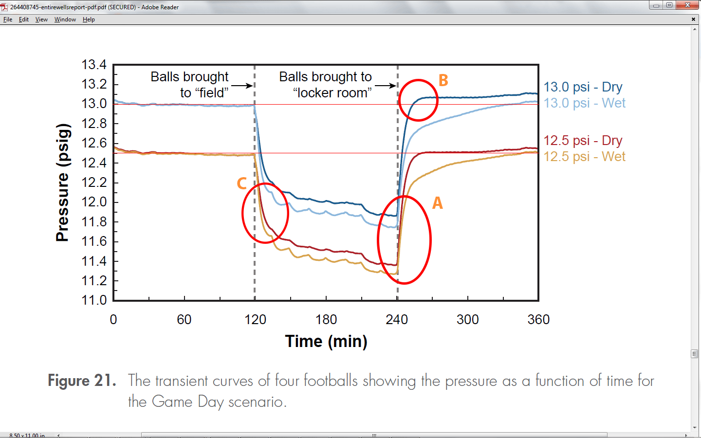
Not surprisingly there is evidence in the Exponent report that the Exponent curves could also have been caused by climate control problems within their chamber. Figure 21 shown above shows the non-exponential behavior as the pressure curves for the dry balls rises too quickly and then abruptly flattens in region B. It also rises and flattens too quickly for the Patriots dry-ball curve (not highlighted). It is hard to speculate what did this without knowing the apparatus, but it certainly is not indicative of a smooth temperature transition.
The Exponent investigators never mention evaporative cooling as being the source of the difference between wet-ball and dry-ball pressures. It is also evident by looking at their charts that they had a hard time with consistency between different runs of the apparatus. In the different charts containing wet balls and dry balls, these range between a separation of .15psi (Fig. 21) to .23psi (Fig. 29) to .46psi (Fig. 27), at the lowest pressure ranges, and we expect that separation to become larger as the balls move into the locker room, with warm dry air (see Chart 21). These should all be the same. The only explanation here is that they had a hard time controlling the humidity in their simulated rooms. At 48F, with 75% humidity, the dry bulb temperature was 45F, corresponding to a separation of .15psi. .46psi is simply too large a separation, and must correspond to a lower humidity.
The few data points they put on the Fig 29 seem to track closely to their experimental wet-ball pressure curve. Of course, you expect they would. The curve was calibrated in the same conditions the balls brought in would be. The bigger question is what that curve would look like in the actual Patriots locker room, with some balls covered in moisture on their entire surface, and the unknown climate control within that setting.
To summarize this discussion of evaporative cooling, there are a number of big areas of concern:
- The calibration and control of the humidity and temperature within the simulation seems to have led to an artificially rapid rise in the pressure as measured during the locker room phase of the simulation.
- Air circulation and humidity during cooling may have caused inconsistent pressure differences between wet and dry balls. From the Exponent data when the ball is simulating being on the field and cooling, it is apparent that there is enough air circulation and dampness on the balls to achieve the wet-bulb temperature/pressure because of the difference in pressures between a dry-ball and a wet-ball at the low point in pressure. However there is no mention of the air circulation or windspeed in the report. By their report, they did try to maintain the humidity at 75%, but the variability in the separation between dry and wet balls suggest they may have had problems controlling this. There should be some uncertainty calculation in the startoff point of the transient curve, or a calibration of the separation between wet and dry balls, that should show up in their report.
- Dampness of the balls. The balls will dry pretty quickly in a warm dry environment (e.g. 72F at 20% humidity). Based on the simple theory of evaporative cooling, the amount of water on the balls could make a large difference in their measurements here, and could be substantially different from what happened during the actual time in the locker room. Some sort of measurement of dampness, and its effect on the curve should be in the report.
The air circulation and evaporative cooling problem greatly confuses the expected temperature rise (and pressure) of a wet ball. We also don’t know how wet/dry the balls were. What percentage of the surface area of the ball was really wet? Did the Exponent drying with a towel really correspond to what the ball boys did on the field? Was there a significant problem with managing the climate control — the humidity and temperature of the simulated locker room? This result from Exponent is at best incomplete in this area, and make it difficult to make conclusions.
Appendix D. Wet Bulb and Dry Bulb Temperatures
Psychromatic Chart — The wet-bulb temperature can be determined using this well known chart. Look for it on the Internet and watch videos on its usage. The lines shown are used to determine the Web Bulb temperatures relevant to the DeflateGate situation.

Appendix E. Control Groups and Calibration (added on later)
Some people have asked about the Colt’s footballs. What happened to them? The Wells Report makes a big point of using them as the “control”.
In an experiment a control group is the group that you don’t perform the experiment on, but in all other ways is like the group you are performing the experiment on. The difference between the control group and the experimental group then shows the effect of the experiment.
In this case the Colt’s balls were considered the control group, and the Patriot’s balls were the experimental group — the experiment being that someone along the way may have deflated the Patriot’s balls. Presumably that was the only difference in their treatment.
But wait a moment. There is a laundry list of differences in their treatment:
- The two groups of balls may have been initially measured with two different pressure gauges, resulting in a .37psi difference right at the beginning.
- Only 4 balls of the Colt’s 12 balls were measured. All the Patriot’s balls were measured.
- Four of the Colts balls had never been used in the game, and were dry. Was it these four that were measured?
- Or were the four those that had been sitting at the top of the bag in the locker room, and most exposed to the warmer air, and least exposed to sitting at the bottom of the bag on the cold turf?
- There special procedures for handling the balls on the ball field taken by the Colts, including putting them in plastic garbage bags to help keep them dry, and potentially less exposed to evaporative cooling.
- The Colts offense sat on the bench for 30 minutes before halftime, and their footballs were less exposed to the weather and the cold field.
- The Colts balls were measured much later at half-time than the Patriots, and there seem to be some issues with measuring what was happening with evaporative cooling during that time.
- How dry did the balls boys for each team really get the footballs?
With all this, and perhaps there is more, it is hard to think of the Colt’s balls as a reliable control group, particularly since, as we have discovered, footballs are quite sensitive to temperature and evaporative cooling.
Because of the uncertainties in the ball handling, I find it more sensible to just evaluate based on the basics laws of physics. And just the simple measurement assuming the Logo gauge was the measuring device and some slowed warming due to evaporative cooling, or some additional cooling due to the cold field seems to put us there.
If you want to use the Colt’s balls as controls, all those differences above need to be accounted for.
It is a dilemma for the Wells investigators however. Without a control group, or without returning to Gillette stadium and doing some calibration measurements in cold weather, all they will have done is proved that their experimental apparatus in Menlo Park, CA differs in a statistically significant way from whatever happened on January 18, 2015 at Gillette Stadium in New England, rather than the other way around.
